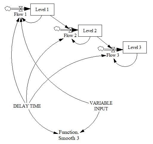
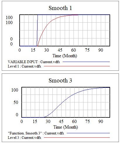
The model shows first and third order delays. The first order produces an exponentially asymptotic curve because the "Level 1" and "Flow 1" loop has a negative sign, this means that the adjustment is reduced over time.
The explanation of why a third order delay leads to a sigmoidal curve can be based on the three steps that require Level 3 to begin the adjustment after 3 periods and not from the change value of the Input variable but rather on the value of Level 2.

Equations
(01) DELAY TIME=30
(02) FINAL TIME = 100
(03) Flow 1= (VARIABLE INPUT-Level 1)/(DELAY TIME/3)
(04) Flow 2= (Level 1-Level 2)/(DELAY TIME/3)
(05) Flow 3= (Level 2-Level 3)/(DELAY TIME/3)
(06) Function Smooth 3=SMOOTH3(VARIABLE INPUT,DELAY TIME )
(07) INITIAL TIME = 0
(08) Level 1= Flow 1,0
(09) Level 2= Flow 2,0
(10) Level 3= Flow 3,0
(11) TIME STEP = 1
(12) VARIABLE INPUT= STEP(100,20)
